Reinforcement Learning for Orbital Transfers at the 2026 AI Winter School (Brown University)
6 min read
Hands-on workshop framing orbital transfer as a controlled two-body dynamics problem: Hohmann benchmark, Gymnasium environment, PPO policies, reward shaping, and diagnostics for chatter and delta-v efficiency.

At the 2026 AI Winter School, hosted by the Center for the Fundamental Physics of the Universe at Brown University, I led a 2.5-hour hands-on workshop on reinforcement learning for orbital transfers.
The workshop was not about claiming that RL is the right way to solve a textbook astrodynamics problem. The point was to use a problem with known mechanics and a known analytic solution as a controlled environment for learning the applied RL workflow: define the state, action, reward, and diagnostics; train a policy; compare it against ground truth; then explain the failure modes.
Control Problem
The notebook used nondimensional two-body dynamics: unit gravitational parameter, an initial circular orbit at radius 1, and a target circular orbit at radius 1.6. I call those radii and below. The model omitted drag, finite-duration thrust, J2 perturbations, third bodies, attitude dynamics, and mass depletion. Control was a tangential impulse applied once per simulation step.
Here the arrowed r denotes the spacecraft position vector; the plain r denotes its scalar radius. The state evolves under central gravity:
That stripped-down model is still useful because the relevant orbital invariants are visible. For a circular target orbit, the target specific energy and angular momentum are known:
The RL environment did not need to know the absolute orbital angle. The observation vector used normalized radius, radial velocity, tangential velocity, angular-momentum error, energy error, and previous action. Removing angle makes the policy rotationally symmetric: the same local orbital state should produce the same control decision anywhere around the planet.
Hohmann Benchmark
Before training PPO, the notebook computed the Hohmann transfer. For circular, coplanar orbits with two impulsive burns, the transfer semi-major axis is:
The two burns and transfer time are:
That closed-form solution gave the workshop a real yardstick: not just “did the agent reach the target,” but how much Δv it spent, how many burns it used, whether it circularized, and whether the trajectory matched the expected burn-coast-burn structure.
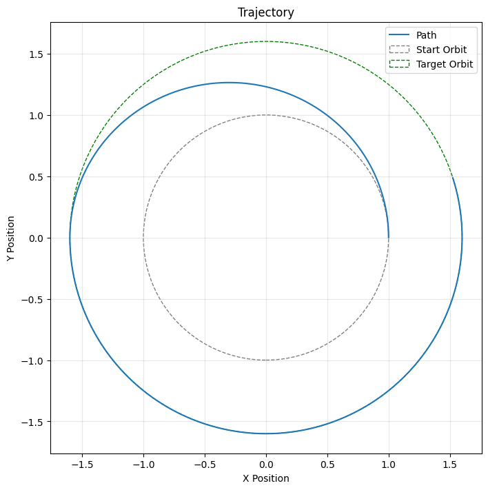
The verification plots made the baseline concrete: the trajectory should be an ellipse touching r1 and r2, the radius history should rise from the inner orbit to the outer orbit after the second burn, and cumulative Δv should match the analytic total.
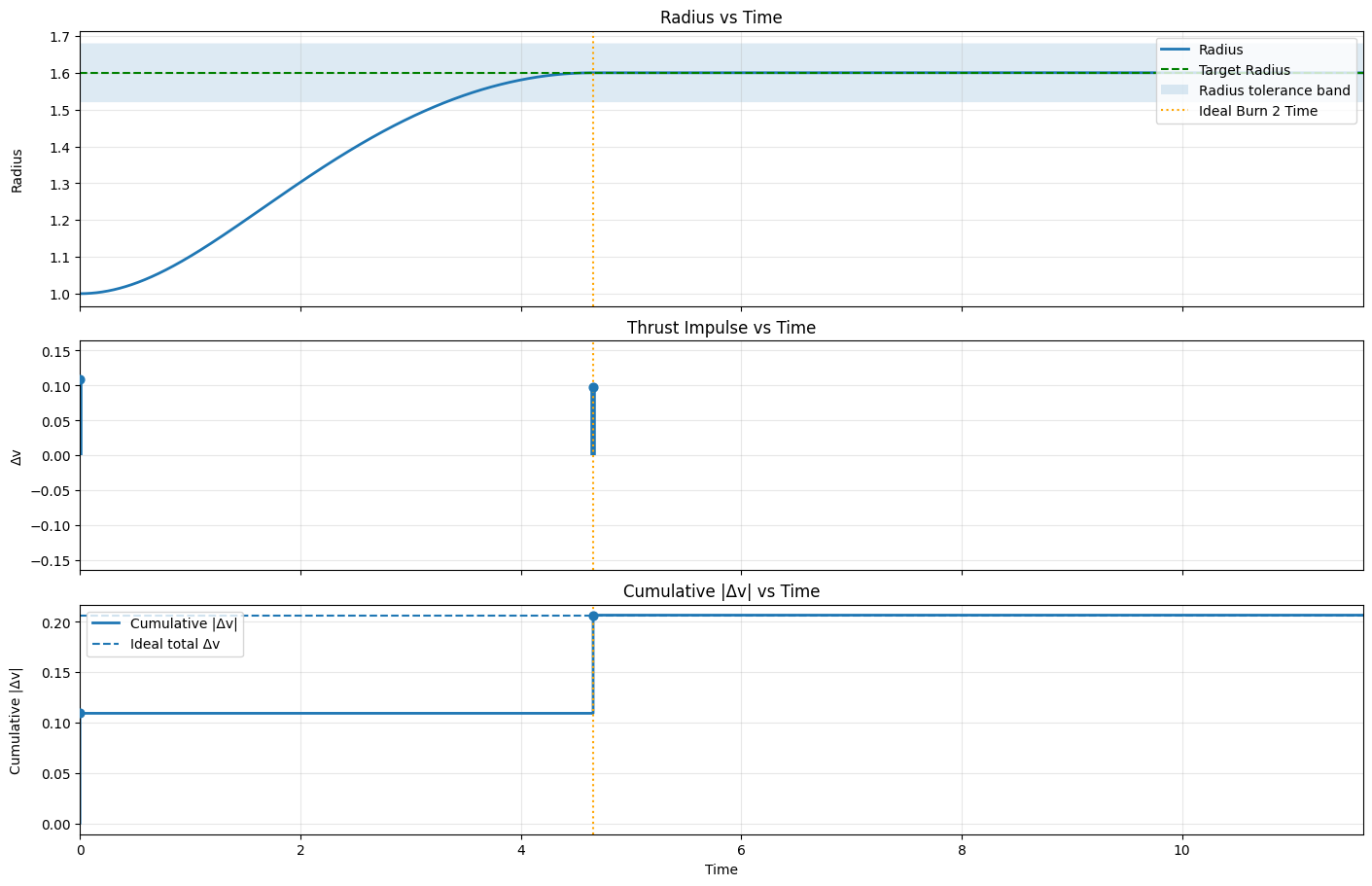
One useful teaching detail appeared immediately: even the analytic plan does not land exactly on r2 in a finite-timestep simulator if the second burn fires on the first step at or after the computed transfer time. The total Δv still matches theory, but the final orbit has a small residual timing error. That separates continuous-time theory, numerical integration, and policy behavior before RL enters the discussion.
Try it: fly the transfer yourself
A normalized 2-D two-body simulator with tangential impulse control. It uses the same mechanics as the workshop notebook: start on r₁ = 1 and circularize at r₂ = 1.6 using as little Δv as possible. The analytic Hohmann transfer needs Δv ≈ 0.207 — try to match it, press Run Hohmann to watch the textbook solution, or Run Greedy to see a myopic controller reach the target the expensive way.
Hold a burn button to keep firing · prograde is along your velocity · a clean transfer is two burns and a coast, not a stream of corrections.
RL Formulation
The Gymnasium environment held the physics fixed and varied the control interface:
| Component | Implementation |
|---|---|
| Observation | Normalized r, vr, vt, target angular-momentum error, target energy error, previous action |
| Discrete action | coast, full prograde impulse, full retrograde impulse |
| Continuous action | throttle in [-1, 1], mapped to a signed tangential Δv impulse |
| Success criteria | tolerances on , , and |
| Failure criteria | crash/escape radius or episode timeout |
The dense reward used a combined energy/angular-momentum error:
with shaping approximately proportional to:
Then the environment subtracted fuel and ignition/switching penalties, added a one-time success bonus on first entry into the tolerance region, and added a holding reward for staying there. PPO was trained with observation/reward normalization during training, frozen normalization statistics during evaluation, and deterministic policy rollout for diagnostics.
What the Diagnostics Caught
The important lesson was that endpoint success is too weak a metric. A policy can enter the success region and still be a poor transfer.
The notebook compared policies using trajectory, radius history, radial velocity, thrust impulses, cumulative Δv, number of burns or active-thrust steps, closest-to-target statistics, and the mission report against the Hohmann ideal.
The failure modes were instructive:
- Discrete control: small fixed impulses can reach the target, but often with many prograde/retrograde corrections. The orbit may satisfy the tolerance band while wasting Δv.
- Continuous control: throttle control is more expressive, but it can learn micro-thrusting: almost continuous small corrections that keep the error low while hiding poor fuel efficiency.
- Tolerance exploitation: a policy can appear to “beat” the ideal by stopping inside loose tolerances on a slightly elliptical orbit. That is not a better transfer; it is a reminder that the metric defines the game.
- Final-state ambiguity: final radius alone is misleading for eccentric orbits. Closest approach, radial-velocity history, angular momentum, and thrust history are needed to interpret what the policy actually learned.
Experiment Loop
The final notebook section let participants edit a ModeConfig and rerun training. The knobs were not decorative; each one changes the control problem:
dv_mag: control authority per stepfuel_cost_penalty: cost of using Δvignition_penalty: cost of turning on or changing thrustreward_shaping_scale: strength of dense energy/angular-momentum shapingtraining_timesteps,learning_rate, andent_coef: PPO optimization and exploration behavior
The practical standard was:
train a policy
inspect trajectory, thrust, and Δv
compare against Hohmann
explain the failure mode
change one parameter or design choice
rerun
That loop is the point of using RL in a problem with analytic ground truth. The goal is not to celebrate a learned policy for reaching the target. The goal is to make the policy’s behavior legible enough that failures are evidence for the next experiment.
Materials
Workshop Recording
Slides
Code
RL for Orbital Transfers Notebook
Event Page
For the full schedule and recordings across all modules: